Visualising Macrobond data as maps using R
You already know how to visualise Macrobond’s wealth of macroeconomic and financial aggregate data using a variety of line, bar and other charts.
But did you know you can also use it to create geographic heat maps in just a few steps?
We take you through the process:
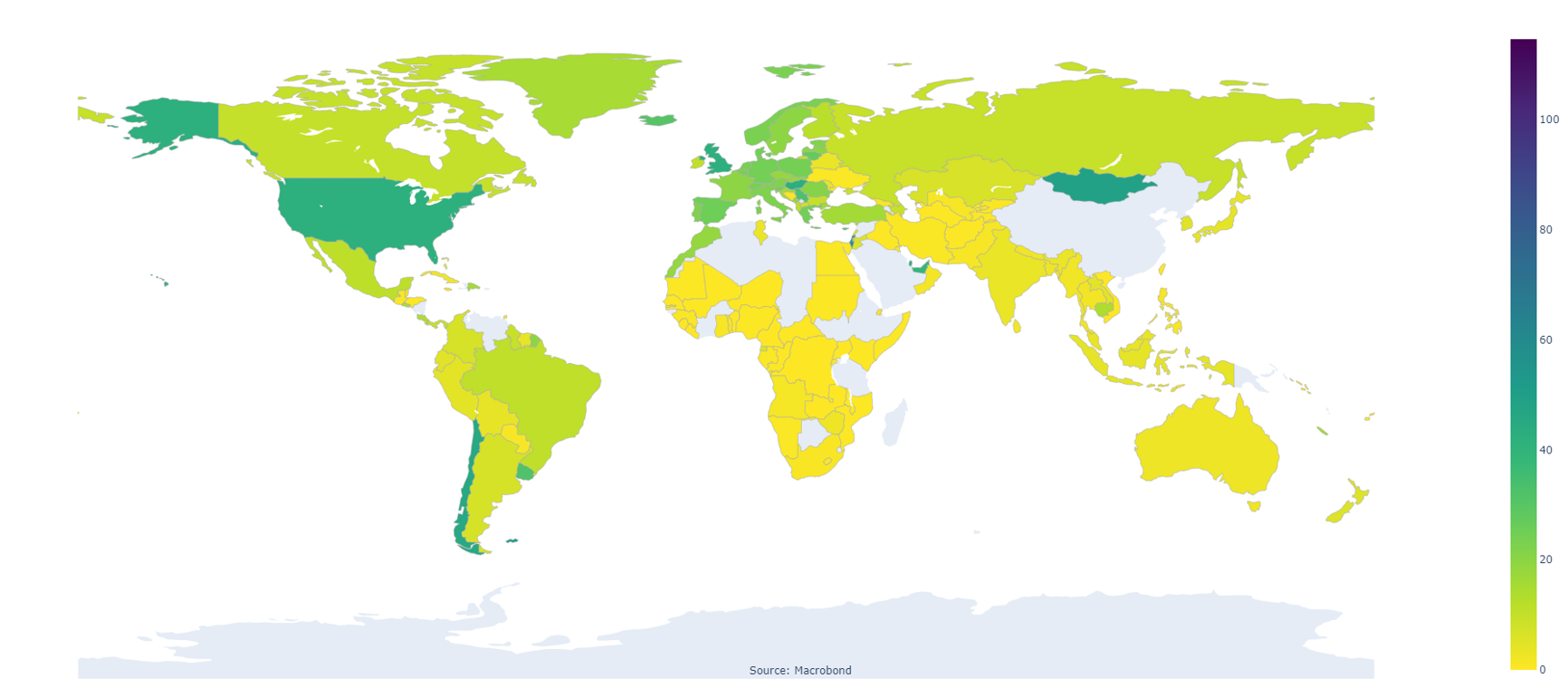
Our World in Data, COVID-19, Vaccinations, People Fully Vaccinated Per Hundred
Step 1: Define some functions to efficiently return the ISO 2 code for the region and return the last value of the series
library(MacrobondAPI)
library(ggplot2)
library(tidyverse)
library(rnaturalearth)
library(rnaturalearthdata)
A function to get the region of the series
GetRegion<- function(entity) getFirstMetadataValue(getMetadata(entity),"Region")
GetRegionNames<- function(entities) sapply(entities, GetRegion)
A function for getting the ISO2 for a country from the region code entity
metaInfoIso <- GetMetadataInformation("IsoCountryCode2")
GetRegionIso2 <- function(entity)
{
regionName <- getValuePresentationText(metaInfoIso, getFirstMetadataValue(getMetadata(entity), "Region"))
}
# A function for getting the last value using the metadata
GetLastValueFromMetadata <- function(entity)
{
getFirstMetadataValue(getMetadata(entity), "LastValue")
}
Step 2: Find the same variable for several countries. Use the search functionality in the Macrobond API for a specific concept. Find this under “Time Series information” in the application or by using the “Get Concepts” function in R.
Getting the concept of a series
series<-FetchOneTimeSeries("owidvacci_ar_pfvph")
concept<-getConcepts(series)
Searching for a concept in Macrobond and accessing the available data globally
query <- CreateSearchQuery()
setEntityTypeFilter(query, "TimeSeries")
addAttributeValueFilter(query, "RegionKey" , concept)
searchResult <- SearchEntities(query)
entities <- getEntities(searchResult)
Step 3: Now create a data frame with the ISO 2 codes and the last value, which can be done through the functions defined earlier.
regionNames <- GetRegionNames(entities) #Getting the Region names from the search result
regionEntities <- FetchEntities(regionNames)#Getting the Region Entities from Region in order to translate it to ISO2
regionIso <- GetRegionsIso2(regionEntities) #Getting the ISO 2
entitiesAndRegions <- mapply(function (entity, iso) c(entity = entity, iso = iso), entities, regionIso) #Converting the ISO
Step 4: Now it’s time to match your dataset with the map. Use rnaturalearth to get the coordinates for the countries on the map and join thatdataset with the Macrobond data.
Inserting the country list for the map from rnaturalearth
mapdata <- ne_countries(scale = "medium", returnclass = "sf")
Remove entries for which we do not have matching iso codes
entitiesAndRegions <- entitiesAndRegions[unlist(sapply(entitiesAndRegions, function(x) !is.null(x$iso) && x$iso %in% mapdata$iso_a2))]
lastValues <- sapply(entitiesAndRegions, function(x) GetLastValueFromMetadata(x$entity))#Getting the last value from the meta data
isoCodes <- sapply(entitiesAndRegions, function(x) x$iso) #Getting the ISO2 codes
Creating a dataframe with region and last value
insert_data <- data.frame(iso_a2 = isoCodes, value = lastValues)
Joining the values with the map dataset
mapdata <- left_join(mapdata, insert_data, by="iso_a2")
mapdata <- subset(mapdata, select = c(name, value, geometry, iso_a2))
Step 5: Now you’re all set to create your map through ggplot.
Creating the map
map <- ggplot(data = mapdata, aes(text = paste(name, "<br>", "Fully vaccinated:", value,"%"))) +
geom_sf(aes(fill = value))+
ggtitle(GetConceptDescription(getConcepts(entities[[1]])))+
labs(title = GetConceptDescription(getConcepts(entities[[1]])), x = "Source: Macrobond")+
scale_fill_viridis_c(name = "%", option = "viridis", trans= "reverse")+
theme(axis.text.x = element_blank(),
axis.text.y = element_blank(),
axis.ticks = element_blank(),
axis.title.y=element_blank(),
rect = element_blank())
.svg)
Using Plotly
If you would like to take this to the next level, you can also use Plotly to create the interactive map.
Creating a widget with plotly
library(plotly)
fig <- ggplotly(map, tooltip = c("text"))
fig
Here’s the full code:
library(MacrobondAPI) #This sample requires Macrobond API 1.2-4 or later
library(ggplot2)
library(tidyverse)
library(rnaturalearth)
library(rnaturalearthdata)
library(plotly)
GetRegion <- function(entity) getFirstMetadataValue(getMetadata(entity), "Region")
GetRegionNames <- function(entities) sapply(entities, GetRegion)
GetLastValueFromMetadata <- function(entity) getFirstMetadataValue(getMetadata(entity), "LastValue")
GetRegionsIso2 <- function(regionEntities) sapply(regionEntities, function(entity) getFirstMetadataValue(getMetadata(entity), "IsoCountryCode2"))
FetchOneTimeSeries()
Searching for a concept in Macrobond and accessing the available data globally
query <- CreateSearchQuery()
setEntityTypeFilter(query, "TimeSeries")
addAttributeValueFilter(query, "RegionKey" , "owdc0008")
searchResult <- SearchEntities(query)
entities <- getEntities(searchResult)
regionNames <- GetRegionNames(entities) #Getting the Region names from the search result
regionEntities <- FetchEntities(regionNames)#Getting the Region Entities from Region in order to translate it to ISO2
regionIso <-GetRegionIso2(regionEntities) #Getting the ISO 2
entitiesAndRegions <- mapply(function (entity, iso) c(entity = entity, iso = iso), entities, regionIso) #Converting the ISO
Inserting the country list for the map from rnaturalearth
mapdata <- ne_countries(scale = "medium", returnclass = "sf")
Remove entries for which we do not have matching iso codes
entitiesAndRegions <- entitiesAndRegions[unlist(sapply(entitiesAndRegions, function(x) !is.null(x$iso) && x$iso %in% mapdata$iso_a2))]
lastValues <- sapply(entitiesAndRegions, function(x) GetLastValueFromMetadata(x$entity))#Getting the last value from the meta data
isoCodes <- sapply(entitiesAndRegions, function(x) x$iso) #Getting the ISO2 codes
Creating a dataframe with region and last value
insert_data <- data.frame(iso_a2 = isoCodes, value = lastValues)
Joining the values with the map dataset
mapdata <- left_join(mapdata, insert_data, by="iso_a2")
mapdata <- subset(mapdata, select = c(name, value, geometry, iso_a2))
library(viridis)
Creating the map
map <- ggplot(data = mapdata, aes(text = paste(name, "<br>", "Fully vaccinated:", value,"%"))) +
geom_sf(aes(fill = value))+
ggtitle(GetConceptDescription(getConcepts(entities[[1]])))+
labs(title = GetConceptDescription(getConcepts(entities[[1]])), x = "Source: Macrobond")+
scale_fill_viridis_c(name = "%", option = "viridis", trans= "reverse")+
theme(axis.text.x = element_blank(),
axis.text.y = element_blank(),
axis.ticks = element_blank(),
axis.title.y=element_blank(),
rect = element_blank())
map
Creating a widget
fig <- ggplotly(map, tooltip = c("text"))
fig